Jev and Calibration: When 90% Should Mean 90%
The forecast for Hobart tomorrow says 70% chance of rain. You read it at 11 pm, standing in the kitchen with the last cup of tea of the day, and you make a decision that will shape your entire Tuesday: the umbrella goes by the door.
Tuesday arrives. It does not rain. Not a drop. The umbrella comes with you to three meetings, a café and the bus, and it stays folded the whole time like a small, bone-dry rebuke. By 5 pm you have composed, in your head, a strongly worded letter to the Bureau of Meteorology. It opens with "with respect", which everybody knows means the opposite.
Here is the thing, though. The forecast was not wrong. It gave a 30% chance of exactly the day you had. If the Bureau said 70% on a hundred days and it rained on all of them, that would be the broken forecast. A 70% forecast promises that, across all the days it says 70%, it will rain on about seven in ten. Tuesday was one of the three.
That promise has a name: calibration. As of September 2026, it is also the main thing a new kind of AI is selling.
On 15 September, a company called TypeSafe released a model called Jev. Jev does not chat and does not write. You give it some data and a typed question ("Which queue should this ticket go to?"), and it gives you an answer from a fixed list, with a probability attached. TypeSafe says those probabilities are calibrated, that "higher confidence means higher accuracy", and that the model "can't hallucinate". Five days later, an independent test team gave it a cake recipe and asked which support queue it belonged in. Jev filed the cake as a technical issue, at 0.94 confidence.
Somewhere, a yoghurt cake is waiting for a firmware update.
Take a deep breath. Jev is not a scam, and a confidence score is not a lie. The cake is a clue. A probability is a promise about a particular population of cases. When a model says 0.94, the useful question is "0.94 about what, exactly?", and whether your cases are in that population.
This matters more than it used to, because Jev's input price is $42 per billion tokens. At that price you stop making a few hundred judgement calls a day and start making hundreds of thousands, and a 2% error rate that was a nuisance becomes a small town of mistakes.
So we will follow the rain forecast down into the machine: what the percentage promises, how a computer is graded on the same promise, and the traps that make an honest number useless. Then a Victorian economist explains why cheap decisions multiply, and a (made-up) support manager runs the test you should run before any model acts on its own confidence.
Leave the umbrella by the door. Let's get into it.
Part 1: What "70% Chance of Rain" Actually Promises
You use a probability forecast almost every day, probably without thinking of it as a statistical instrument. The Bureau of Meteorology is refreshingly direct about it: "Weather forecasts describe likelihoods, not certainties." It counts rain from 0.2 mm, a threshold based on the rain gauge it uses.1 And its own community research found that when it talks about a chance of rain, many people ignore the percentage and focus on the word "rain". So "20% chance" arrives in the brain as "it might rain", when the more useful reading is "it will very probably stay dry".
The US National Weather Service corrects two other misreadings: 40% does not mean rain for 40% of the day, or over 40% of the area. It means a 40% chance of measurable rain at the forecast point. None of that tells you whether the forecaster is any good, which is the interesting question.
One forecast can never be wrong. A thousand can.
You cannot check a single probability forecast. If it says 70% and it rains, the forecaster was right. If it stays dry, the forecaster was also right, because 30% is not zero. This is very convenient for forecasters and deeply unsatisfying for anybody holding an umbrella.
The only test is to collect a lot of them. Take every day the forecaster said 70% and count how many were wet. If the answer is close to 70%, their 70% means what it says. Then repeat for 10%, 20%, 30% and so on.
In 1977, Allan Murphy and Robert Winkler did exactly that. They called the property reliability, and they defined it with a lovely plain example: if a forecaster said 30% on 50 occasions, that set of forecasts "would be perfectly reliable if precipitation occurred on exactly 15 of the occasions". Machine learning people now call the same property calibration. Same idea, different department.
Then they checked real forecasters: every rain forecast from the National Weather Service office in Chicago, July 1972 to June 1976, 17,514 in all. On the 1,574 occasions the forecasters said 30%, it rained on 449, or 28.5%. When they said 70%, it rained about 67% of the time. They ran slightly high at most levels, but across four years of Chicago weather, the numbers held.
I love this result, and not only because people in the 1970s tallied four years of wet days so that a man in Tasmania could make a point about AI in 2026.2 It shows that calibration is a skill with a feedback loop. A forecaster says a number every day, and every day the sky marks their work, with no argument and no six-month wait. Few human experts get feedback that fast. Remember that, because it is the environment you have to build for a machine before you trust its numbers.
What a calibrated number gives you
A calibrated forecast lets you set a rule once and trust the long-run result. You decide what chance of rain is worth an umbrella, and follow that rule. Some days you carry it for nothing. Over a season, you get wet about as often as you chose to. That is the whole value of a calibrated probability: you can set a threshold and trust what the threshold does over many cases. The rest of this article is about how that trust is measured, and how it breaks.
Part 2: How a Machine Is Graded on the Same Promise
A classifier is any model that sorts things into categories: spam or not spam, which support queue, which invoice code. Most modern classifiers produce a probability for every possible answer, and the highest one wins. A model might look at a support ticket and return billing 0.84, technical 0.16. The 0.84 is the model's confidence.
The test is the one the Chicago forecasters passed. Across all the tickets where the model said about 0.84, was it right about 84% of the time? A widely cited 2017 paper by Chuan Guo and colleagues, On Calibration of Modern Neural Networks, states it almost exactly as Murphy and Winkler did: given 100 predictions, each with confidence of 0.8, "we expect that 80 should be correctly classified". The weather clerks and the machine learning researchers arrived at the same test forty years apart.
Bins and the reliability diagram
A model does not say exactly 0.8 a hundred times, so you group predictions into bins, usually ten of equal width: 0.0 to 0.1, 0.1 to 0.2, and so on up to 0.9 to 1.0. (The Chicago forecasters got this step for free, because they were only allowed to use certain round numbers.) For each bin, you work out the average confidence and the accuracy, which is the share of predictions in that bin that were correct.
Then you plot them: confidence along the bottom, accuracy up the side, and a diagonal line from corner to corner. That chart is a reliability diagram.
- Points on the diagonal: the model means what it says.
- Points below it: the model is overconfident. It says 0.9 and is right 75% of the time.
- Points above it: the model is underconfident. It says 0.6 and is right 80% of the time.
The Guo paper found that the neural networks of 2017, though far more accurate than older ones, had become worse at this. A deep 110-layer network got more answers right than a small 1998-era one, but its confidence was "substantially higher than its accuracy". Better at the job, worse at knowing when it was wrong. (I have worked with consultants like this. Once or twice, I have been one.)
ECE: the chart as one number
A chart is good for a person. A dashboard wants a single number, and the usual one is Expected Calibration Error (ECE). It sounds intimidating. It is an average of gaps:
- For each bin, take the gap between accuracy and average confidence.
- Weight each gap by the share of all predictions that sit in that bin.
- Add them up.
An ECE of 0 means every bin sits on the diagonal. An ECE of 0.10 means the model's confidence is, on average, about ten percentage points away from how often it is right.
Two warnings. ECE depends on your bins: change from 10 to 15 and the number moves. And it is never exactly zero on a real sample, because small samples are noisy. A careful tester works out the noise floor, the ECE a perfectly calibrated model would still score on a sample that size, and compares against that instead of against zero.3
The Brier score, which weather people invented first
Long before neural networks, a meteorologist named Glenn Brier proposed a way to score probability forecasts, in 1950. For each forecast, take the probability you gave, subtract what happened (1 if it happened, 0 if not), and square it. Then average across all forecasts. It is the mean squared error of the forecast, and lower is better.
Say 0.7 and it rains: (0.7 − 1)² = 0.09. Say 0.7 and it stays dry: (0.7 − 0)² = 0.49. Confident and wrong costs much more than cautious and wrong. In 1973, Allan Murphy (him again) showed that it splits into three parts:
- Reliability: how close your probabilities are to the observed frequencies. This is calibration.
- Resolution: how well your forecasts separate the wet days from the dry ones. This is what makes a forecast useful.
- Uncertainty: how hard the weather was to predict in the first place. You cannot control this one.
Keep resolution in mind. It rescues us from the first trap in Part 4.
A real example from a very large model
Here is the most useful chart I know on this topic. In the GPT-4 Technical Report, OpenAI published two reliability diagrams side by side, for a set of multiple-choice questions. The pre-trained model, before any tuning for conversation, had an ECE of 0.007: almost perfect. After post-training, the process that turns a raw model into a polite assistant, the ECE was 0.074. OpenAI's caption is blunt: "The post-training hurts calibration significantly."
So the raw model knew, quite precisely, how likely it was to be right, and the training that made it pleasant to talk to made it worse at knowing. That is the gap Jev says it fills. To see why, look at how a chat model produces an answer at all.
Part 3: Fast Thinking, Slow Thinking and a Machine That Writes One Word at a Time
TypeSafe calls Jev a "System One Model", after Daniel Kahneman's Thinking, Fast and Slow. In Kahneman's framing, System 1 is fast, intuitive and emotional, and System 2 is slower, more deliberative and more logical. System 1 knows, instantly, that the kettle has boiled. System 2 works out how many cups of tea you drink in a year.4
It is a clever name, and TypeSafe is candid about its catch. Its FAQ admits that "System 1 thinking" has also implied error-prone, because System 1 is the part of us that jumps to conclusions. TypeSafe says it believes these models can be made more reliable than the alternatives, and promises to explain why later.
How a chat model answers: one token at a time
A large language model does not decide an answer and then write it down. It writes to find out what the answer is. I went through the machinery in AI Hallucinations 101. The short version: the model sees text as tokens (pieces of words), predicts a probability for every possible next token, picks one, adds it to the text and repeats. TypeSafe's comparison table puts it well: "Generates one token at a time, each conditioned on the last."
So when you ask a chat model "Is this email phishing?", the probability you care about is buried in its choice of the first few tokens. When you then ask "How confident are you, from 0 to 100?", you do not get that probability. You get the model writing a number, token by token, like anything else it writes. TypeSafe's table says that even when prompted, these models "tend to be overconfident and inconsistent", and the GPT-4 chart shows one reason why.
In Kahneman's terms, you asked for a quick gut call, and the machine answered with a slow essay about its gut.
How Jev answers: the whole distribution at once
Jev takes a different route. You send it some state (the ticket, the email, the invoice) and one or more typed questions. As MarkTechPost summarises from the docs, there are three types:
- Noul: is this statement true? It returns one probability from 0 to 1.5
- Choice: pick one option from a list of up to 255. It returns the winner and a probability for every option.
- Score: rate against ordered levels (for example, how urgent a ticket is).
TypeSafe says Jev "outputs all probabilities in parallel instead of autoregressively generating by token", and that it is trained with a method it calls Reinforcement Learning for Calibrated Decisions (RLCD), aimed at "epistemically honest probabilities". It has not published the architecture or the weights, so everything else has to be measured from the outside.
The design idea is sound. If you want a probability over a fixed set of answers, a model that returns it directly is a better fit than one that writes an essay and hopes the probability survives. It is also much faster: TypeSafe quotes 70 ms to 500 ms per response, which it puts at "40x-200x faster" than frontier chat models on the same kind of task.6
What "can't hallucinate" actually means
Here the marketing and the mechanism part ways, and TypeSafe, to its credit, says so on the same page. The claim is that Jev "can't hallucinate". The note underneath, in TypeSafe's own words: "Our number is not empirical. Schema matching is guaranteed, thus we can confidently add 0% into the plots."
In plain terms: ask Jev to choose between billing, technical and account, and it always returns one of those. It never invents a fourth queue called "Tuesday". Anybody who has found "Certainly!" where a JSON bracket should be will appreciate that.
But an answer can be the right shape and still be wrong. The cake's output was perfectly valid, and it was nonsense. A schema guarantees that the answer comes from your list, not that it is the right item on the list. So when a vendor says "cannot hallucinate", translate it as "cannot return an invalid type", then go looking for the calibration evidence, because that is where any claim about correctness has to live.
As of September 2026, that evidence does not come from TypeSafe. AgentConn's review notes that TypeSafe has published "no reliability diagram, no expected calibration error (ECE) and no ablation". TypeSafe's published workflow evals measure accuracy, and they measure it against "consensus labels": the average answer of two other AI models, GPT-6 Astra and Fable 5.1, not human-checked truth. On that measure Jev scored 67.8%, level with GPT-5.6 Terra (67.9%) and behind Sol (74.1%)7, at a tiny fraction of the cost and time. In its launch post, TypeSafe notes that its own team built the workflows, so "some bias could exist". That is a fair caveat, and an invitation to check. So independent people did.
Part 4: Four Ways a Calibrated Score Still Fools You
Within a week of launch, several developers published their own tests of Jev. None is peer reviewed; each is one small team, one setup, one week, and the model may have changed since. As a set, though, they show every classic calibration trap in the wild.
Trap 1: Calibrated and useless (the base-rate forecaster)
Meet the laziest forecaster in history. We will call him Barnaby. Barnaby has noticed that in Chicago it rains on about one day in five. (Murphy and Winkler give the climatological probability as about 0.20.) So Barnaby says "20% chance of rain" every single day, whatever the sky is doing. Blue sky: 20%. Black clouds and thunder: 20%. A flood rising over the next paddock: 20%, and could someone pass him a biscuit.
Over a year, it rains on about 20% of the days Barnaby says 20%. His reliability diagram has one point, on the diagonal, and his ECE is close to zero. By the calibration test alone, Barnaby is world class. He is also useless, because he never tells you anything you did not already know. Barnaby's reliability is perfect and his resolution is zero, because his forecasts do not separate wet days from dry ones. As the Brier score reference puts it, when the climatological probability is always forecast, "the resolution is zero". Meteorologists call Barnaby's forecast "climatology" and use it as the no-skill baseline that any real forecaster must beat. (In machine learning you will often hear the related idea called sharpness: how often a model is willing to commit to a probability far from the average.)
AgentConn reports a community test in which Jev screened adverts for scams. The ECE was a respectable 0.046. But at a 0.9 threshold, Jev acted on only 8 adverts and caught 7 of the 53 scams. In AgentConn's words: "A calibrated score, and no usable threshold." The number was honest. It rarely said anything confident enough to act on.
A low ECE is necessary and nowhere near enough. You also need the model to be confident often, and right when it is.
Trap 2: Calibration shifts with the data
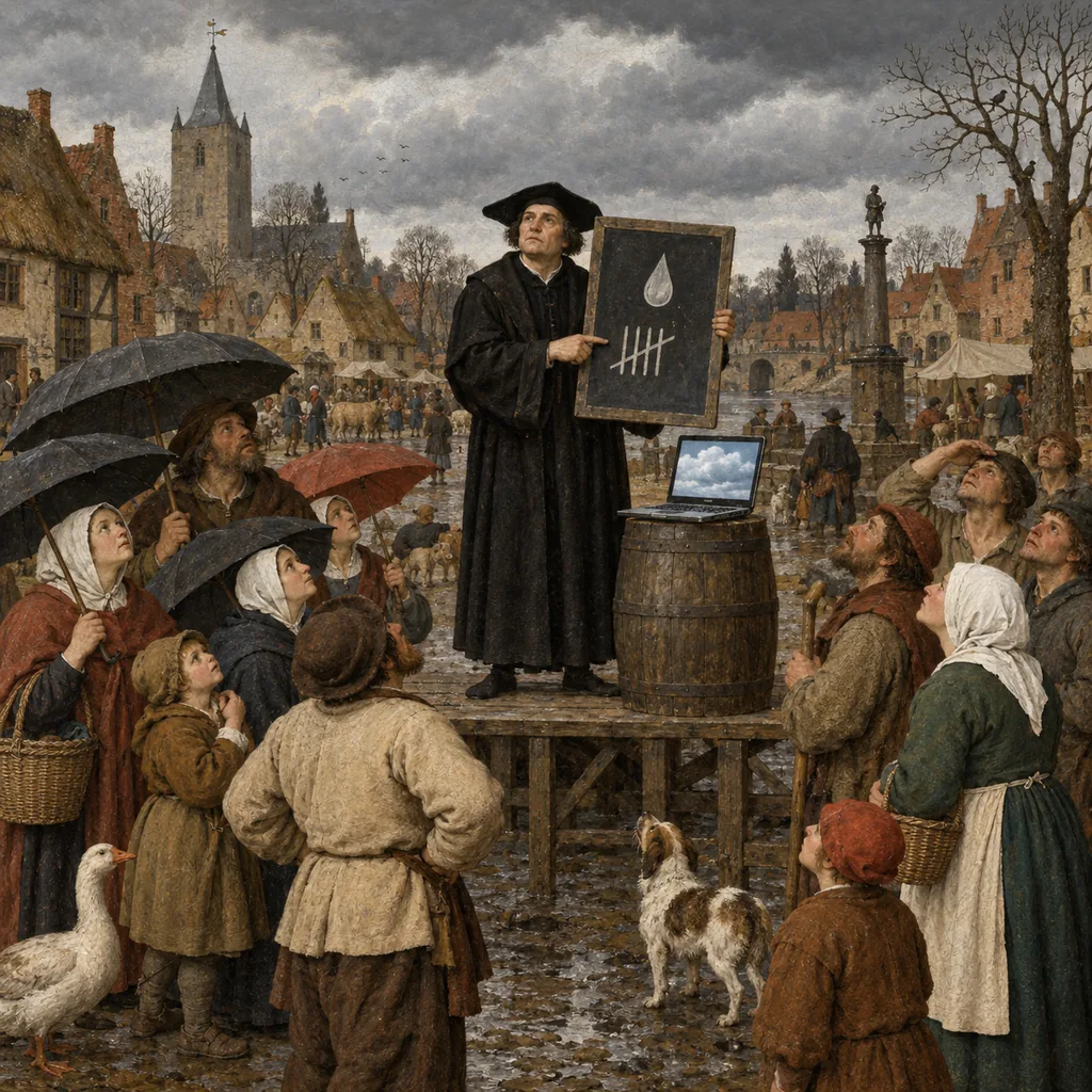
The Chicago forecasters were calibrated on Chicago weather. Send them to Hobart for a winter and their 30% would mean little until the sky had marked a few months of their work. Calibration belongs to a forecaster on a particular kind of day.
The clearest Jev test of this comes from a developer who publishes as scienthoon. They ran Jev on public benchmarks, standard test sets that a model might well have seen in training, and found an ECE of 0.024 to 0.032. Close to perfect. Then they generated 900 new synthetic support tickets that Jev could not have seen, and asked three questions about each. The ECE rose to 0.107, which they measured at 4.4 times the noise floor for a sample that size.
The yes-or-no questions came out underconfident: Jev was right more often than it said. The Choice and Score questions came out overconfident: right less often than it said. The author warns that the size of the error depends on technical choices in the fit, and gives advice I would like printed on a tea towel: "Read the sign, not the magnitude." The same model, on the same day, was too humble on one kind of question and too sure on another.
TypeSafe's own documentation agrees, which I respect. Its page on Jev's weak spots says: "Don't carry a threshold tuned on a Noul over to a Choice." It also reports that a question and its exact negation got probabilities of 0.72 and 0.47. Those should add up to 1. They add up to 1.19. Each question has its own calibration, and you have to measure each one.
Trap 3: Confident about the unanswerable
One of scienthoon's three questions had a trick in it. Ticket priority was partly set by an internal rule based on the customer's tier, and that rule never appeared in the ticket text. Nobody, human or machine, could reliably get the answer from the text alone. Jev was right 44.7% of the time (chance was 25%), and its chosen answer carried an average probability of 0.74.
That is Barnaby turned inside out. Facing an impossible question, a well-calibrated model should give low, flat probabilities. Jev said "fairly sure" and was wrong more often than right. Part of the reason applies to any model that must choose from a list. As Langfuse put it in their testing notes, Jev "cannot abstain". Give it only billing, technical and account, and it must pick one. PriorBench showed where that leads: "Without an explicit 'none of these' option, 0 of 30 out-of-scope messages were flagged", and those misfiled messages still came back at very high confidence. A separate PriorBench test fed it meaningless input: that is where the cake came from, and a string of random letters went the same way, at 0.97. Calibration is measured against the question you asked. If your list has no "this doesn't belong here", the model's confidence is confidence about the wrong question.
Trap 4: Option order, and other things that should not matter
Ask the same question with the same options in a different order. Nothing about the ticket changed, so the answer should not change. For chat models, we have known for a while that it does. A 2023 study by Pouya Pezeshkpour and Estevam Hruschka found that simply shuffling the answer options produced a performance gap of about 13% to 75% across benchmarks. Their explanation: when a model is torn between two or three answers, a small bias towards a position tips it.
Jev is not immune. PriorBench's advice is to "Fix your option order for ambiguous tasks (up to 13 points of movement)." Borderline cases, exactly where you want a trustworthy probability, are where order moves the result.
Two smaller cousins turned up too. Jev also returns a separate confidence field, which sounds like the better number to threshold on; in scienthoon's tests it was never better than the top probability, and their advice is: "Don't threshold on the confidence field." And the gateway they used exposed no model version, so the model "may move silently". A calibration result describes one version. If it changes without you knowing, your threshold is a guess.
And one trap that is really a cliff
PriorBench found one more shape worth knowing. On their main test, accuracy above each threshold was flat from 0.50 to 0.95, then jumped to 100% above 0.99, a band that covered 60.2% of the traffic. Raising the bar from 0.5 to 0.95 bought almost nothing. Raising it to 0.99 bought everything. That is less a slope than a cliff. Their advice: "Gate at 0.99, or do not gate."
That may not hold on your data, which is the point. You do not know the shape of your model's reliability diagram until you draw it on your own decisions.
In fairness: what the tests say about accuracy
Jev is not a dud. On PriorBench's 400-item main test, Jev scored 95.9% with no training, against 77.2% for hand-written keywords. In a phishing test on 2,000 emails, asked the single question "is this phishing?", Jev scored 62.6% against 81.3% for Claude Haiku 4.5. Clearly worse. But when the author split the question into five narrow ones (does the link use a URL shortener? does a free email address claim to be a company?) and fitted a small statistical model on the answers, Jev reached 95.0% and Haiku 93.2%, a gap the author found not statistically significant. A simple pattern-matching rule scored 91.8%, because in that dataset the links carry most of the signal. As Beri's write-up says, that 95% is Jev plus labelled data plus a regression you maintain, not Jev alone.
The same phishing test found Jev about 12 times cheaper than Haiku ($0.038 against $0.462 per 1,000 emails) and about 2.9 times faster, measured from France. TypeSafe's headline of "193.6x faster, 444.6x cheaper" comes from its own workflows, which it says are "on the higher end of real world gains". Different tests, different places. According to MarkTechPost, Guillermo Rauch of Vercel has also reported Jev up to 18x faster at p95 than GPT Luna, and more accurate.
So, as of September 2026: very cheap, very fast, strong on narrow questions, weaker on broad ones, and with confidence scores that carry real information but are not textbook-calibrated on new data. That is a useful tool. It is a tool that needs you to do the checking.
Part 5: Jevons' Paradox, or Why Cheap Decisions Multiply
Jev is named after William Stanley Jevons, a Victorian economist; TypeSafe's launch announcement calls the name "a nod to Jevons Paradox". It is a better name than most AI companies manage, and it carries a warning.
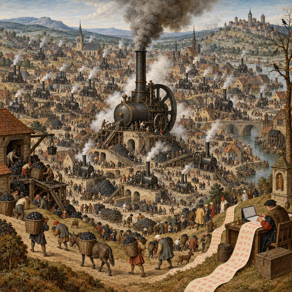
In 1865, Jevons published The Coal Question. Britain was worried about running out of coal, and one popular hope was that more efficient steam engines would save it. Jevons argued the opposite. If an engine uses less coal per unit of work, coal-powered work gets cheaper, so people do much more of it, and total coal use goes up. In his words: "It is wholly a confusion of ideas to suppose that the economical use of fuel is equivalent to a diminished consumption. The very contrary is the truth."
TypeSafe makes the same prediction for AI: "Every order of magnitude drop in the cost of intelligence unlocks orders of magnitude more use cases." I think they are right. That is exactly why calibration becomes the thing that matters most.
The arithmetic of cheap mistakes
PriorBench ran their whole test suite, 5,721 calls, for $0.176. TypeSafe's Doom demo makes 10 queries a second, about 36,000 an hour, for roughly $7 an hour. At those prices, nobody asks whether a decision is worth an AI call. Now watch the errors. These numbers are round and made up, to show the shape:
- A team makes 200 judgement calls a day by hand, with a 2% error rate. That is 4 mistakes a day, and somebody usually notices each one.
- The same judgement is automated and applied to everything, 200,000 times a day, at the same 2% error rate. That is 4,000 mistakes a day, and nobody notices most of them.
Same error rate, a thousand times the errors. That is Jevons' paradox, with mistakes in place of coal.
It compounds when one decision is split into several steps, as TypeSafe recommends. If each of five steps is independently right 98% of the time, all five are right about 90% of the time (0.98 to the power of 5). Five good decisions make one mediocre pipeline.
This is where calibration earns its keep. If you cannot make every decision right, the next best thing is to know which ones are probably wrong and send those to a person. At a fraction of a cent per decision, the model is not the expensive part. The mistakes you did not catch are.
For a real number: in the phishing test, Jev's single-question approach flagged 18.0% of legitimate emails as phishing. At 10,000 legitimate emails a day, that is 1,800 innocent emails in quarantine every day, from a model that costs almost nothing to run.
Part 6: Ingrid Runs a Shadow Test
Meet Ingrid. Ingrid runs the support desk at a mid-sized software company in Launceston. (She is made up. Launceston is real, and I will defend its honour.) Her team routes about 400 tickets a day into four queues: billing, technical, account and sales. A person reads each ticket and picks a queue. Her manager has seen the Jev pricing and would like it switched on by Friday.
Ingrid would like that too, but only for the tickets it will get right. So she runs a shadow-mode test: the model sees real work and answers, but its answer changes nothing. A person still decides, and you compare the two afterwards.

Monday: gather the labelled decisions
Ingrid exports 1,600 tickets from the last month. For each one she keeps the final queue, the one the ticket ended up in after any reassignment. If a ticket went to billing first and was moved to technical, the right answer is technical. If she used the first guess, she would be grading Jev against her own team's mistakes.
She checks the sample is fair: a normal month, not the outage week, with the odd ones left in (spam, job applications, and one message that just says "hello?"). (This is the construct validity question from Are You Really Tracking That?: make sure the thing you measure is the thing you mean.)
Tuesday: write the question like code
She writes one Choice question: "Which team should handle this ticket?" The options are billing, technical, account, sales and none of these. The fifth option is the lesson of the cake.
She writes one clear line of description for each option, because PriorBench found that wrong option descriptions were "catastrophic", worse than random. She sends only the ticket subject and body, because TypeSafe's docs say accuracy falls as the state fills with detail the question does not need. She fixes the order of the options and never changes it, and she pins a specific model version.
Wednesday: run it in shadow and split the data
She runs all 1,600 tickets through Jev and stores every probability, including the losing options. Then she splits the tickets at random into two halves of 800: a tuning half and a test half. She will choose her threshold on one and check it on the other, so she is not marking her own homework.
On the tuning half, she sorts predictions into bins by top probability and works out the accuracy in each. These figures are invented for Ingrid, to show the method:
| Confidence bin | Tickets | Average confidence | Accuracy | Gap |
|---|---|---|---|---|
| Below 0.5 | 15 | 0.42 | 0.33 | 0.09 |
| 0.5 to 0.6 | 30 | 0.55 | 0.50 | 0.05 |
| 0.6 to 0.7 | 45 | 0.65 | 0.58 | 0.07 |
| 0.7 to 0.8 | 70 | 0.75 | 0.66 | 0.09 |
| 0.8 to 0.9 | 120 | 0.85 | 0.80 | 0.05 |
| 0.9 to 1.0 | 520 | 0.97 | 0.93 | 0.04 |
Every bin sits a little below the diagonal, so on Ingrid's tickets Jev is slightly overconfident. The ECE is the weighted average of the gaps, (15 × 0.09 + 30 × 0.05 + 45 × 0.07 + 70 × 0.09 + 120 × 0.05 + 520 × 0.04) ÷ 800, or about 0.049. Fairly good, but Ingrid cares more about whether any band is good enough to act on.8
Thursday: find the band that clears the bar
Ingrid's team agrees an accuracy bar with the people who own the queues. A misrouted ticket costs about a day, so automatic routing must be right at least 98% of the time. The top bin is right 93% of the time. Not good enough.
So she looks inside the top bin. The 330 tickets at 0.99 or higher are right 98.5% of the time. That clears the bar, and it covers 330 of 800 tickets, about 41%.
Then the important step. She applies the rule "auto-route at 0.99 or higher" to the untouched test half. There, 326 tickets reach 0.99, and 98.2% of them are right. The rule holds on data it has never seen.
For every ticket, the system records the state Jev saw, all the probabilities, the model version, the rule applied, the action and the final human queue. That log is how Ingrid will know, six months from now, whether the model has drifted.
Friday: switch on the part that earned it
Ingrid switches on automatic routing at 0.99 or higher. Everything below still goes to a person, now with Jev's suggestion filled in. Each week she re-runs the reliability table on the latest labelled tickets.
Her manager asks why only 41% is automatic when the model is "95% accurate". Ingrid shows him the table and says one sentence: "The 41% is the share we can prove." He goes to make a cup of tea, which is the correct response to a well-made table.
The next week he asks whether Jev can also do refunds, invoice coding and churn risk: Jevons' paradox, in person. Ingrid says yes, each with its own shadow test, because a threshold tuned on routing tells you nothing about refunds.
What to Do This Week
You do not need Jev for any of this. The checks work on any model that gives you a probability. (If you read my guide to bias in AI, this is the same discipline: measure on your data, not the vendor's.)
- Pick one high-volume decision that already has answers. Ticket routing, invoice coding, alert triage, lead scoring. You need records where you know the final, correct outcome.
- Export 1,000 to 2,000 labelled records. Use the final human outcome, not the first guess, and make sure the strange cases are in the sample.
- Write the question like code. Add a "none of these" option to every Choice. Write clear option descriptions, fix the option order and send only the fields the question needs.
- Pin the model version and store it with every result.
- Run the model in shadow. Store every probability for every record. Let it change nothing.
- Split the records into two random halves. Tune on one, test on the other.
- Draw the reliability diagram on the tuning half, with 10 equal-width bins. A spreadsheet is enough: top probability in one column, 1 or 0 for right or wrong in the next, averaged per bin.
- Calculate ECE and the Brier score, and count what sits in the confident bins. A good ECE with nothing confident is Barnaby.
- Agree an accuracy bar with the people who own the decision, then find the band that clears it. The share of records in that band is your real saving.
- Confirm the band on the test half. If it fails there, it is not a rule yet.
- Threshold on the probabilities, not on a separate
confidencefield, unless your own test shows that field is better. Tune each question separately, and never reuse a threshold across question types. - Compare cost per correct decision, not cost per token, against what you do now. Include what the mistakes cost.
- Re-run the table on a schedule, and every time the model version or your inputs change.
And one check for the next sales meeting. When a vendor says their model "cannot hallucinate", ask three questions. Where is your reliability diagram? On what data? And what does the model do when the right answer is not on my list?
Final Thoughts
Think back to the umbrella on a dry Tuesday. The forecast did its job. If anything failed, it was the reading of the number.
That is the lesson from Jev. A probability is a promise about a long run of cases, never a single one, and it is worth something only once it has been checked on cases like yours, by someone who is not selling it to you. Weather forecasters earned trust in their percentages because the sky marked their work every day. An AI model has to earn the same trust the same way, and as of September 2026, the marking is up to you.
Jev may turn out to be a very good tool, cheap and fast enough that you will be tempted to use it everywhere. If Jevons is right, you will. So before your decisions multiply, pick one decision, export a thousand labelled examples and draw one reliability diagram. It will tell you more about your model than any launch post.
Now, if you'll excuse me, the Bureau says there is a 70% chance my tea is ready. On current form, I like those odds.
Notes
-
The Bureau ties the 0.2 mm figure to the rain gauge it uses. Anything below that does not count as rain for forecasting purposes, however damp your washing feels. ↩
-
The Chicago forecasters could only use set values: 0%, 2%, 5%, 10%, 20% and then steps of 10% up to 100%. That limit made the results easy to tabulate. It also means nobody in Chicago was ever told there was a 37% chance of rain, which feels like a loss for the city. ↩
-
A perfectly calibrated model tested on a small sample still shows gaps in each bin, from chance alone. Testers usually estimate the noise floor by simulating a perfectly calibrated model on the same number of predictions and measuring the ECE it scores. ↩
-
About 1,820 cups, or five a day. I did the System 2 work once, so that System 1 can reach for the kettle without guilt. ↩
-
Noul is TypeSafe's name for a yes-or-no question. Langfuse's testing notes point out that a Noul answer has no separate confidence field, only the probability, so code that expects a confidence value on every answer will break on yes-or-no questions. ↩
-
DataCamp's write-up of the launch gives TypeSafe's speed range as "40x-200x" in its introduction and "20-200x" in its summary. The TypeSafe launch post itself says 40x to 200x. ↩
-
The evals page labels its two OpenAI comparison models only "terra" and "sol". TypeSafe's launch post names GPT-5.6 Terra, and OpenAI released its GPT-5.6 family, including Sol, on 9 July, but the evals page itself does not spell the names out. ↩
-
With only 800 predictions, some bins in a table like Ingrid's hold very few tickets, so their accuracy can swing by several points from chance alone. Merging the smallest bins, or showing the count in each, keeps a small sample from telling a bigger story than it can support. ↩