A Nobel for Neural Networks: Backpropagation Without the Maths Panic

On Tuesday evening I was halfway through a cup of tea when the Nobel Prize in Physics appeared on my screen, and I read the citation twice. It was "for foundational discoveries and inventions that enable machine learning with artificial neural networks". In physics. Not computer science, which has no Nobel Prize, but the prize that has gone to the electron, the neutrino and the Higgs boson. This year it went to John Hopfield and Geoffrey Hinton, for work that most people meet as a chatbot, an image search or the thing that guesses the next word on their phone.

I assumed somebody in Stockholm had been hacked. Then on Wednesday the chemistry prize arrived, and half of it went to two people from Google DeepMind for AlphaFold, an AI model that predicts the shapes of proteins. At that point I started to plan for the rest of the prizes. Literature to autocomplete, "for sentences that are statistically likely". Peace to whichever chatbot apologises the most. Economics to the algorithm that sets surge prices.

The best detail of the week, though, came from the winner himself. The Nobel Prize website calls new laureates for their first reactions, and in that phone call, Hinton said he was "in a cheap hotel in California, without an internet connection", where it was "two o'clock in the morning". He had no idea he had even been nominated. His very first thought was "how could I be sure it wasn't a spoof call". What convinced him was that the person "had a strong Swedish accent and there were several of them". That is better identity checking than most banks manage: one Swedish accent can be faked, but a whole committee of them is a lot of effort for a prank.¹

Asked whether he was a computer scientist or a physicist, Hinton said he was "someone who doesn't really know what field he's in but would like to understand how the brain works". That is a better answer than any of my jokes.

So, settle down. The physics department has not been hacked, and you do not need a maths degree to follow this. The prizes are a good excuse to learn the one idea that sits under almost every AI product you use, and that the committee's own background paper names in the middle of its story: backpropagation. It is the procedure that lets a neural network learn from its mistakes. And it has a reputation as calculus that sensible people avoid, which is a pity, because it is mostly multiplication and a fair way of sharing out blame.

Here is the plan. First, what the two prizes were actually for, because the headlines blurred it. Then we build a neural network from parts you already use: one artificial neuron, then a score for how wrong it is, then a walk downhill in thick fog, then backpropagation itself, with a two-weight example small enough to do on the back of a teabag packet. Then a made-up analyst called Marnie trains one in a spreadsheet, and I give you a short list of things to try this week.

Let's get into it.

Part 1: What the Prizes Were Actually For

The physics press release has a heading that tells you how the committee sees it: "They trained artificial neural networks using physics". The physics in question is the physics of magnets and of systems made of many small parts. Neither laureate won for ChatGPT. Both won for work from the 1980s that the field built on.

The Hopfield network: memories as valleys

In April 1982, John Hopfield published a short paper in PNAS with the wonderful title "Neural networks and physical systems with emergent collective computational abilities". He described a network that worked as a content-addressable memory. In plain words: you find a memory by giving it part of the memory, not an address. The abstract says it "correctly yields an entire memory from any subpart of sufficient size".

You do this all day. Somebody hums three notes and you have the whole song. You did not look up "song number 4,127". The fragment pulled out the whole.

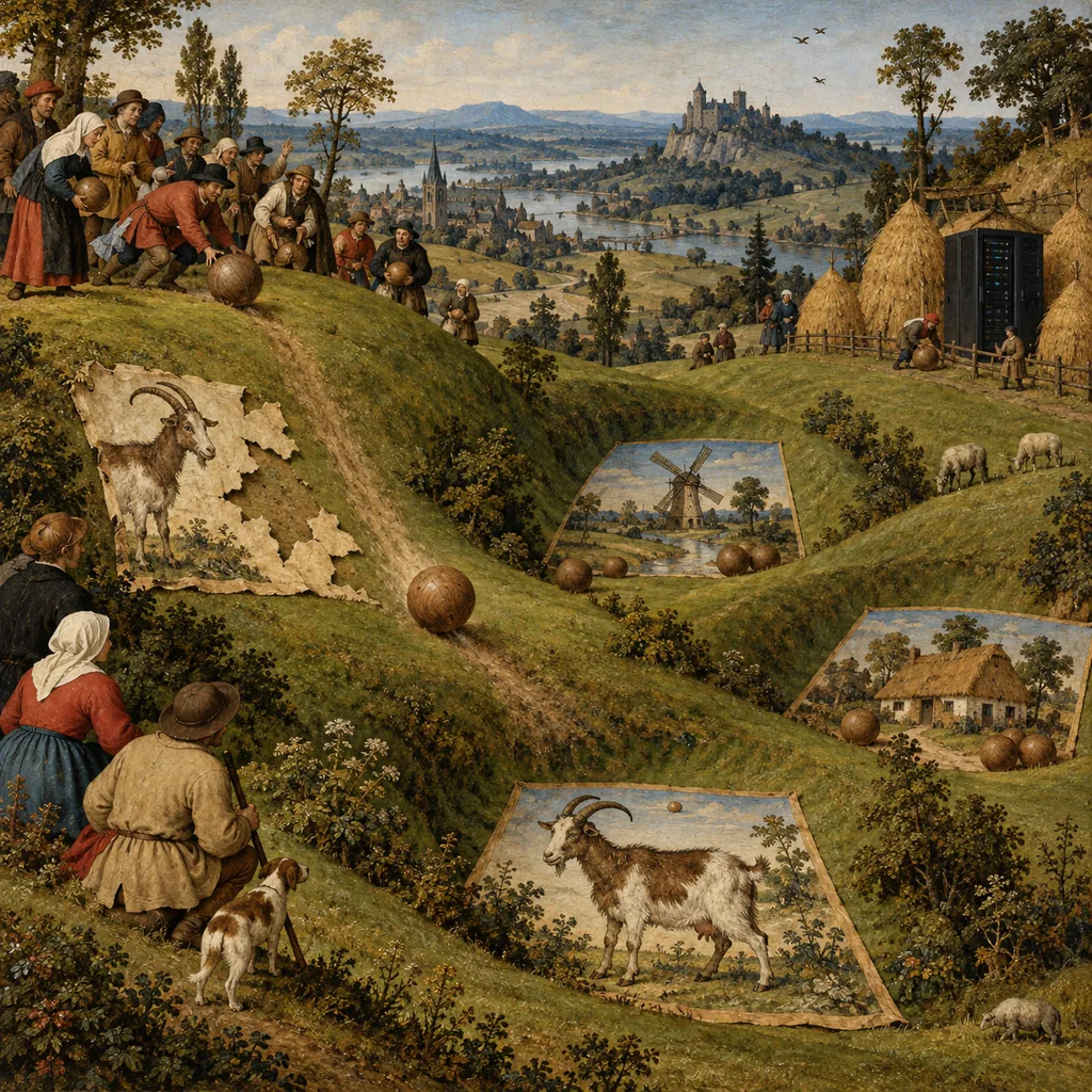
Hopfield's network does the same with simple on-off units, which you can think of as the pixels of a black-and-white picture. Every unit is connected to every other unit, and each connection has a strength. To store a picture, you set the strengths so that the stored picture has a low energy, a number borrowed from the physics of magnetic materials, where each atom behaves like a tiny magnet that affects its neighbours. To recall a picture, you give the network a damaged copy, and it changes one pixel at a time, always in the direction that makes the energy fall, until no change helps any more. The committee's popular explanation describes the result in a picture that Hopfield used himself: a ball rolling through "a landscape of peaks and valleys", with friction. Each stored memory is a valley. Drop a damaged picture on the slope and it rolls into the nearest valley, which is the closest stored picture. The scientific background puts it more formally: the dynamics drive the system "to the valleys of an N-dimensional energy landscape", and those valleys are the memories.

Keep that ball in mind. Rolling downhill to the bottom of a valley is going to come back, wearing a different hat, in Part 4.

The scale is charming. According to the popular background, Hopfield's 1982 network had 30 nodes, so 435 connections and "fewer than 500 parameters". He tried 100 nodes, but that was too much for the computer he had.² The committee compares that with today's large language models, which "can contain more than one trillion parameters".

max_tokensPOST./v1/messages

The Boltzmann machine: the same valleys, with dice

Between 1983 and 1985, Hinton, with Terrence Sejnowski and others, extended Hopfield's idea into the Boltzmann machine. The name comes from Ludwig Boltzmann, the nineteenth-century physicist whose equation describes how likely a system is to be in each of its possible states at a given temperature. Hinton's network makes its moves with a bit of randomness, set by a pretend temperature, and it has hidden units: units that are not part of the input or the output, free to represent whatever helps. Instead of storing particular pictures, it learns the general pattern of a kind of data, so it can recognise new examples, or produce new ones of the same kind. The committee notes that the full version was "initially of limited use" in practice, because each learning step needed slow simulations, and that a slimmed-down version, the restricted Boltzmann machine, became the useful tool. In the 2000s, Hinton used it to pre-train deep networks layer by layer, then fine-tuned them "using the backpropagation algorithm". That is the first time backpropagation shows up in our story, and it will not be the last.

The chemistry prize: AlphaFold and designed proteins

The chemistry press release split the prize in two. Half went to David Baker, at the University of Washington, "for computational protein design". In 2003, his group designed a new protein "unlike any other protein", and since then it has produced many more. The other half went jointly to Demis Hassabis and John Jumper of Google DeepMind "for protein structure prediction".

Proteins are long strings of amino acids that fold into three-dimensional shapes, and the shape decides what the protein does. Predicting the shape from the string had been, in the words of the chemistry committee's chair, Heiner Linke, a "50-year-old dream". In 2020, Hassabis and Jumper presented AlphaFold2. At the blind CASP14 competition that year, DeepMind reported a median score of 92.4 GDT, against a level of about 90 that is "informally considered to be competitive with results obtained from experimental methods". The committee says AlphaFold2 has now predicted the structure of "virtually all the 200 million proteins that researchers have identified", and has been used by "more than two million people from 190 countries".³

And not everybody clapped

It would be odd to write about AI credit without mentioning an argument, and this week has one. Jürgen Schmidhuber, a researcher who has argued for years that deep learning credits the wrong people, posted on X the next day:

The #NobelPrizeinPhysics2024 for Hopfield & Hinton rewards plagiarism and incorrect attribution in computer science. It's mostly about Amari's "Hopfield network" and the "Boltzmann Machine."

[…]

— Jürgen Schmidhuber (@SchmidhuberAI), 9 October 2024 on X

The post goes on, as a numbered list, to argue that Shun-Ichi Amari described an adaptive network of this kind in 1972. I am not going to settle a forty-year argument about credit in one blog post. But it is useful to know that the history of these ideas is crowded, and you will see this again with backpropagation itself. The committee's own background is careful on that point.

So that is the history. Now the useful part: how does any of this actually learn?

Part 2: One Neuron, Built From a Saturday Morning

Start with a decision you make without thinking. It is Saturday morning in Hobart, and you are deciding whether to go to Salamanca Market. You consider three things. Is it raining? Do you need vegetables? Did a friend say they would be there? You do not weigh these equally. Rain counts strongly against. Needing vegetables counts a fair bit for. The friend counts a little for, depending on the friend. You also start with a general mood: some people are market people, and they need very little reason to go.

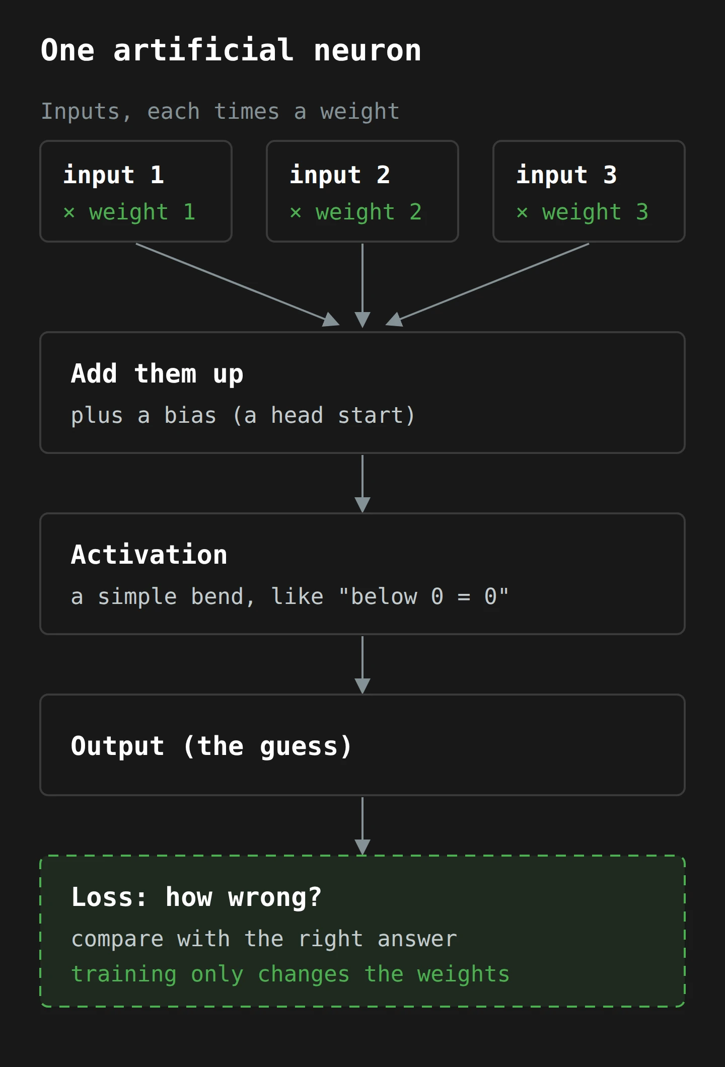
You just did a weighted sum. Each input (rain, vegetables, friend) is multiplied by how much it matters to you (its weight), you add them up, you add your general mood (a bias), and if the total is over some line, you go.

That is almost exactly what an artificial neuron is. In 1943, the neuroscientist Warren McCulloch and the logician Walter Pitts proposed a model in which a neuron "formed a weighted sum of binary incoming signals", and that sum decided its output. A modern artificial neuron does the same thing with ordinary numbers:

1. Multiply each input by its weight.
2. Add them up, and add the bias.
3. Pass the total through an activation function, a simple bend. A common one today just says: if the total is below zero, output zero; otherwise, output the total.⁴
4. The result is the neuron's output.

There is nothing clever in that list, and that is the point. The cleverness is entirely in the weights. A neuron with good weights makes good decisions. A neuron with random weights makes random ones. Learning, for a neural network, means one thing: changing the weights. Hold on to that sentence, because everything else in this article serves it. The neuron is the computer version of your Saturday morning decision.

stop_reasoneval:.pass

From one neuron to layers

One neuron can only draw one line. In 1957, Frank Rosenblatt built a network for recognising images, in hardware, with three layers of units but adjustable weights only between the last two. It worked on simple problems, but it could not handle what the committee calls the "one or the other but not both" problem, known as XOR.⁵ In 1969, Marvin Minsky and Seymour Papert spelled out these limits in an influential book, which the committee says "led to a hiatus funding-wise" for the whole field.

The fix was known in principle: put more layers of neurons between the input and the output. These are hidden layers, and they let the network build its own in-between ideas. For example, the first layer might learn "edge here", the next "corner here", and the next "probably an ear". The problem was that nobody had a practical way to train them. If the network's final answer is wrong, which of the thousands of weights, many layers back, should change, and by how much?

That question is the whole subject of the rest of this article. To answer it, we first need a way to say how wrong "wrong" is.

Part 3: Loss, or a Number for "How Wrong"

You cannot improve what you cannot score. A loss function (or just loss) is a rule that takes the network's guess and the right answer and gives back one number: zero if the guess is perfect, bigger the further off it is.

The simplest useful one is squared error: take the guess, subtract the right answer and square the result. Guess 3 when the answer is 2, and the loss is (3 − 2)², which is 1. Guess 5, and it is 9. Squaring does two things. It makes every miss positive, so a miss too high and a miss too low do not cancel out. And it punishes big misses much more than small ones.

Across a whole set of training examples, you average the loss. That average is the single number that training tries to push down. The 1986 backpropagation paper describes it almost word for word: the procedure "repeatedly adjusts the weights of the connections in the network so as to minimize a measure of the difference between the actual output vector of the net and the desired output vector".

Here is the uncomfortable part, and it matters more for you than any of the calculus. The loss is the only thing the network ever cares about. It does not know what you meant. It knows what you measured. If your training data has a bias, the network will faithfully learn the bias, because that is what lowers the loss (I went through how that happens in Decoding Bias in AI). And if your loss measures something slightly different from what you want, you will get a very well-trained answer to the wrong question. In conversion rate work, I call that a construct validity problem (Are You Really Tracking That? is the long version). Machine learning has the same problem, with more decimal places.

So now we have a network with weights and a single number that says how badly it is doing. The question becomes very concrete: which way should each weight move to make that number smaller?

Part 4: Gradient Descent, or Walking Down kunanyi in the Fog

Picture yourself near the top of kunanyi / Mount Wellington, the mountain behind Hobart, on one of those afternoons when the cloud comes down and you cannot see your own boots.⁶ You want to get down to the city. You have no map and no view. What do you do?

You feel the ground. You test the slope under your feet in each direction, find the direction that goes down most steeply, and take a step that way. Then you stop, feel the ground again, and take another step. Repeat until every direction goes up. You are now at the bottom of something.

That is gradient descent, and it is the method that trains almost every neural network in use. Here is the translation, piece by piece:

• Your position on the mountain is the current set of weights. With two weights, the mountain has two directions, like a real one. With 175 billion weights, as GPT-3 has, it has 175 billion directions. Nobody can picture that, and nobody needs to, because the method does not change.
• Your height is the loss. Low is good.
• The slope under your feet is the gradient: for each weight, how much the loss changes if that weight moves a tiny bit, and in which direction.
• Your step size is the learning rate. Take giant strides and you will leap straight over the valley and land on the opposite slope, higher than you started. Take tiny shuffles and you will still be on the mountain at Christmas.

This is the same downhill roll as Hopfield's ball in Part 1, used for a different job. Hopfield's network rolls downhill on an energy surface to recall a memory. A trained network walks downhill on a loss surface to learn its weights. Systems that settle into their lowest energy state are home ground for physicists, and I suspect that is part of why the committee saw this work as physics.

The fog analogy also explains the most famous worry about the method. You might walk confidently down into a small hollow halfway down the mountain, find that every direction goes up, and stop there, convinced you are in the city. That is a local minimum. How much of a trap it is in a network with millions of directions is a story for another post.

Feeling the slope, the slow way

So how do you feel the slope? The obvious way is to nudge. Take one weight, move it up by a tiny amount, run the network again, and see how much the loss changes. The change divided by the nudge is the slope for that weight. Then put it back, and do the same for the next weight. And the next.

This works. It is also hopeless. One nudge per weight means one full run of the network per weight, per step. AlexNet, the image network we will meet in Part 7, had 60 million parameters. Feeling the slope by nudging would take 60 million runs of the network for every single step down the mountain, and training takes a very large number of steps. You would still be standing in the fog when the sun burns out.

What we want is a way to get the slope for every weight at once, for roughly the cost of running the network once more. That is backpropagation.

page_viewtool_use

Part 5: Backpropagation, or Passing the Blame Back Up the Line

utm_source=SELECT

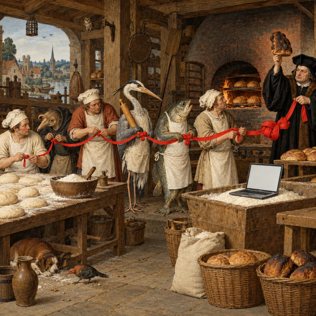
Imagine a small bakery with a production line. The mixer mixes, the shaper shapes, the oven person bakes, and at the end an inspector tastes the loaf and gives it a score. Today's loaf is bad. Whose fault is it?

A sensible bakery does not fire everyone, and it does not shout at the mixer only because the mixer is first. It works backwards. The inspector says the loaf is too dense, by this much. The oven person says: "given what I received, my part of that is small, and most of the density was already in the dough I was handed." So the blame passes back to the shaper, with an exact amount attached. The shaper does the same sum and passes the rest of it back to the mixer. Each person only needs two things: the blame handed to them from the next person in line, and how much their own step changed the result. Multiply those, and you have their share. Pass it on.

We have started down this bakery story, so we are now committed to it. That backward pass is backpropagation. In the jargon: backpropagation applies the chain rule from calculus backwards through the network, from the loss to every weight. Schmidhuber, on his own history page, describes it in one line, and for once I have no quarrel with him. The chain rule itself goes back to Leibniz in 1676. Backpropagation, he says, is "the efficient way of applying the chain rule to big networks with differentiable nodes".

The chain rule, without the panic

The chain rule sounds frightening. It is something you already do with exchange rates.

Say (made-up round numbers) one Australian dollar buys two units of a currency called the Fish, and one Fish buys three Biscuits. How many Biscuits does a dollar buy? Two times three: six. You did not need to think about the whole chain at once. You multiplied the rate at each link.

The chain rule says the same thing about change. If changing A by a little changes B by twice as much, and changing B changes C by three times as much, then changing A changes C by six times as much. In a network, each link is a step: a weight multiplied by an input, a neuron's bend, the loss at the end. Each step knows its own local rate of change, and that is easy to work out because each step is simple. To find how the loss depends on any weight, you multiply the local rates along the path from that weight to the loss.

Now the clever bit, which is the whole reason the method matters. If you start from the loss and walk backwards, every weight shares most of its path with its neighbours. So you work out the shared part once and reuse it, exactly as the bakery's shaper reused the inspector's verdict instead of tasting the loaf again. A 2018 survey of the method by Baydin and colleagues gives the result in plain terms: one backward pass gives the slope for every input, where the forward approach needs one pass per input, at the cost of "a small constant factor of overhead". In other words, the slope for 60 million weights costs about as much as a small number of ordinary runs, not 60 million of them.

The whole thing, with real numbers

Here is the smallest network that shows the idea. It is two neurons in a chain, with no bend, so we can watch every number. One input, x, goes into the first neuron, which multiplies it by weight w1 to give a middle value h. The second neuron multiplies h by weight w2 to give the guess, y. The loss is squared error against a target.

Start with x = 2, w1 = 0.5, w2 = 3, and a target of 2.

Forward pass (make a guess).

• h = 0.5 × 2 = 1
• y = 3 × 1 = 3
• loss = (3 − 2)² = 1

The guess is 3, the answer is 2, and we are 1 away, squared.

Backward pass (share the blame). Start at the end and walk back, multiplying the local rates as you go.

1. How does the loss change with the guess? For squared error, the rate is 2 × (guess − target) = 2 × (3 − 2) = 2.
2. How does the guess change with w2? The guess is w2 × h, so the rate is h, which is 1. Multiply by what was handed back: 2 × 1 = 2. That is w2's share of the blame.
3. How does the guess change with h? The rate is w2, which is 3. Multiply: 2 × 3 = 6. That is the blame handed back to the first neuron.
4. How does h change with w1? The rate is x, which is 2. Multiply: 6 × 2 = 12. That is w1's share.

So the slope for w1 is 12, and the slope for w2 is 2. The first weight gets six times the blame of the second, because it is further from the output and its effect is multiplied by everything after it. This is the bakery's backward pass, with numbers attached, and it tells us how much each weight should change.

aria-labelgtm.js

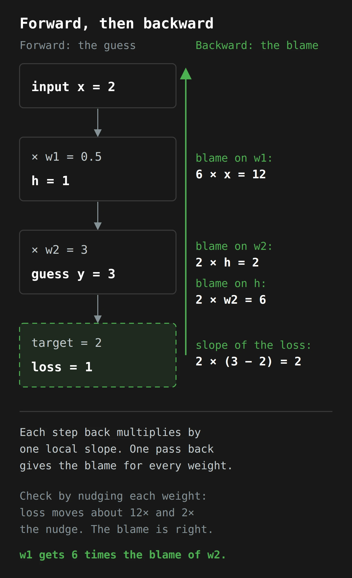
Don't trust me: check it the slow way from Part 4. Nudge w1 from 0.5 to 0.5001 and run the network again, and the loss rises by almost exactly 12 times the nudge. Nudge w2 from 3 to 3.0001 instead, and it rises by almost exactly 2 times the nudge.⁷ The backward pass got both answers from one trip, with no nudging. With two weights, that saves you one run. With 60 million, it saves you the rest of your life.

Take a step downhill. Each weight moves against its slope, by the slope times the learning rate. With a learning rate of 0.01:

• new w1 = 0.5 − (0.01 × 12) = 0.38
• new w2 = 3 − (0.01 × 2) = 2.98

Run it forward again: h = 0.76, y is about 2.265, and the loss falls from 1 to about 0.07. Two more rounds of forward, backward, step, and the loss is about 0.0055, then about 0.0004. The guess is now within a whisker of 2. Nobody told the network which weights to use. It felt the slope and walked downhill.

That is all of it: forward pass, loss, backward pass, small step, repeat. A large modern model does exactly these four moves, with many more weights and much more data.

Who invented it?

This is where Schmidhuber's complaint has a point, and the committee says so too. The 1986 paper by David Rumelhart, Geoffrey Hinton and Ronald Williams, "Learning representations by back-propagating errors", made the method famous. But the Nobel background states plainly that they "reinvented a scheme" that "had previously been applied to related problems by others", and it cites Seppo Linnainmaa (1970) and Paul Werbos. The Baydin survey traces the same mathematics further back, to control theory work of around 1960, and notes that machine learning "reinvented" the method several times. It is a crowded family tree: the same method turned up in more than one field between the 1960s and the early 1980s.

What the 1986 paper did show was something more interesting than the arithmetic. Its abstract says that, as the weights adjust, the hidden units "come to represent important features of the task domain". Nobody told the hidden layer what to look for. The blame did. In the committee's words, they showed "that networks with a hidden layer could be trained by this method to perform tasks known to be unsolvable without such a layer". That was, in effect, the answer to the limits Minsky and Papert had described.⁸

Part 6: Marnie Trains a Network in a Spreadsheet

GPC:.1await

Meet Marnie. Marnie is a data analyst at a mid-sized council in the north of the state. (She is made up. The council is not any particular council, and I would like to keep it that way.) Her manager has just read about the Nobel Prizes and asked, in front of the whole team, whether "the AI" can be trusted. Marnie does not know. So she spends a week building the two-weight network from Part 5 in a spreadsheet, one column per step, because she wants to see it with her own eyes before she answers.

Monday: the forward pass. She makes columns for x, w1, w2, h, y, the target and the loss. Row 1 has x = 2, w1 = 0.5, w2 = 3, target 2. The formulas give h = 1, y = 3 and a loss of 1. The spreadsheet records one row: the weights, the guess and the score.

Tuesday: the slow slope. She adds two columns that nudge each weight by 0.0001 and recompute the loss. The slopes come out at about 12.004 and 2.0001. She notes that each nudge needed its own full copy of the forward calculation, and does the sum in her head for a network with a million weights.

Wednesday: the backward pass. She adds four columns for the backward pass: 2 × (y − target), then times h, then times w2, then times x. They give 2 and 12, the same answers as Tuesday's nudges, with no extra forward runs. Then two more columns for the step: new w1 = w1 − 0.01 × 12, and new w2 = w2 − 0.01 × 2. She copies the row down. The loss column reads 1, 0.0701, 0.0055, 0.0004. She is, for a moment, quite moved by a spreadsheet.

Thursday: the learning rate. Feeling bold, she changes the learning rate from 0.01 to 0.1, to make it learn ten times faster. The loss column now reads 1, 35, 133, 1,315. The network did not learn faster. It took one giant stride over the valley, landed higher on the other side, felt an even steeper slope there, took an even bigger stride, and kept going. This is the most common way real training goes wrong, and it is why the step size has its own name. She changes it back.

Friday: the answer she did not expect. After a few hundred rows at 0.01, the guess is 2 to several decimal places. She looks at the final weights: w1 is about 0.336 and w2 is about 2.975. That is odd, she thinks, because w1 = 1 and w2 = 1 would also work, and so would w1 = 0.25 and w2 = 4. Any pair that multiplies to 1 is perfect. The network did not find the answer. It found an answer, the nearest one to where it started. In this tiny network, the valley floor is a long, flat curve, not a single point. In a large network, it is vastly more so, which is one reason nobody can read a model's weights and say what each one "means".

The following Monday, Marnie gives her manager a better answer than yes or no. "It learns by making its guesses score better on the data we give it, using the score we choose. So the questions are: what data, what score, and how did it do on examples it never saw?" Her manager asks if there will be a spreadsheet. There is a spreadsheet.

Part 7: From 1986 to Your Phone

If backpropagation was famous in 1986, why did it take until the 2010s for neural networks to take over? The committee's popular background says the machine learning revolution "started around 2010", made possible by "vast amounts of data" and "the enormous increase in computing power". Gradient descent is patient, but it is hungry. It needs a lot of examples and a lot of arithmetic.

In the meantime, the method kept working quietly. The scientific background notes that from the mid-1990s, convolutional networks trained by backpropagation, from Yann LeCun and colleagues, were reading handwritten digits on cheques for several American banks.

Then came 2012. Alex Krizhevsky, Ilya Sutskever and Hinton trained an image recogniser, now usually called AlexNet, with 60 million parameters and 650,000 neurons. It took five to six days on two NVIDIA GTX 580 graphics cards. In that year's ImageNet competition, it got a top-5 error rate of 15.3%, against 26.2% for the next best entry. When the ACM gave Hinton, LeCun and Bengio its Turing Award for 2018, it said this result "almost halved the error rate for object recognition and reshaped the computer vision field". The same citation says, quite simply: "The backpropagation algorithm is standard in most neural networks today."

From there, the numbers grow fast. Hopfield's 1982 network had fewer than 500 parameters. AlexNet had 60 million. GPT-3, which I wrote about in AI and the Future of Tech, had 175 billion. The Nobel committee puts today's large language models at "more than one trillion". Every one of those weights got its value the same way as w1 in Marnie's spreadsheet: a forward pass, a loss, a backward pass, and a small step downhill, repeated a very large number of times.

That is also why the chemistry prize belongs in the same story. The physics committee's background calls AlphaFold "the most spectacular scientific breakthrough using deep learning ANN methods". The physics prize rewards some of the ideas the field grew from. The chemistry prize rewards one of the most useful things it has grown into.

What the prize does not tell you

One last thing. In his phone call, Hinton said he hoped the prize would "make me more credible when I say these things really do understand what they're saying". In the same call, the interviewer noted that he had "very publicly expressed fears" about the technology, and Hinton spoke about the need for much more safety research. He clearly hopes the prize gives those warnings more weight. That is a fair thing to want. But notice what the mechanism above does and does not tell you. It tells you how a network gets its weights. It does not tell you what the network has learned, whether it learned what you hoped, or how it will behave on data unlike its training data. Marnie's valley-floor discovery is the small version of that problem. Interpretability, the study of what is going on inside a trained network, is its own active field, and a Nobel Prize does not settle it either way.

What to Do This Week

You can understand neural networks better than most people in a meeting in about an evening. Here is how I would spend it.

1. Do the two-weight example by hand. Use the numbers from Part 5: x = 2, w1 = 0.5, w2 = 3, target 2. Write out the forward pass, the four backward steps and one update. Then check the slopes by nudging each weight. If your numbers match (12 and 2, then a loss of about 0.07), you have done backpropagation. Everything else is scale.
2. Build Marnie's spreadsheet. One row per step, columns for the forward pass, the backward pass and the update. Copy it down 300 rows and chart the loss column. Then try a learning rate of 0.1 and watch the chart leave the page.
3. Play with the TensorFlow Playground. Its own heading is "Tinker With a Neural Network Right Here in Your Browser", followed by "Don't Worry, You Can't Break It. We Promise." Both are true. Pick the spiral dataset, start with no hidden layers, and watch it fail. Add hidden layers and neurons until it succeeds. Push the learning rate up until it falls apart. You will see Minsky and Papert's problem, and its solution, in about two minutes.
4. Watch the backpropagation lesson from 3Blue1Brown. "What is backpropagation really doing?" is the best visual explanation I know, and it starts from the intuition before it reaches the calculus.
5. If you write code, read micrograd. Andrej Karpathy's micrograd is "a tiny Autograd engine" that implements backpropagation in about 100 lines, with a small neural network library of about 50 lines on top. It is the bakery line in Python.
6. Ask three questions of any AI vendor. What is the model trained to minimise (the loss)? On what data? And how did it score on data it never saw during training? A vendor who cannot answer the first question in plain words does not understand their product as well as Marnie does.
7. Check your own measures. If your organisation trains or fine-tunes anything, write down what the loss measures, then write down what you actually want. If those two sentences are different, that difference is where your problems will come from.

Final Thoughts

In the small hours of Tuesday morning, in a cheap hotel in California, a man who says he doesn't really know what field he's in got a call from several Swedish accents and decided, on balance, that it was real. The prize he won rewards ideas from the 1980s: memories as valleys, networks that settle downhill, hidden units that learn their own features. The method that turned those ideas into the AI on your phone is the backward pass you just did by hand.

If you take one thing from this week's prizes, take this: a neural network learns by making a guess, scoring how wrong it was, and handing each weight its share of the blame, then stepping a little way downhill. It is a walk down a mountain in the fog, one careful step at a time, with very good bookkeeping. Once you see that, you know the right questions to ask about any model: what is it walking down, on what data, and how far did it get?

So this weekend, open a spreadsheet, put in x = 2, w1 = 0.5 and w2 = 3, and walk it down the mountain. It takes about ten rows to make the idea stick.

Now, if you'll excuse me, my tea has gone cold while I nudged w2 by 0.0001 for the fourth time. I can feel the slope from here, and it points to the kettle.

Notes

1. Hinton also said he had planned to get an MRI scan that day, and guessed he would have to cancel it. A Nobel Prize is one of the few excuses a hospital booking system has to accept. ↩

2. If every one of 30 nodes connects to every other node, you get 30 × 29 ÷ 2 = 435 connections. Add each node's own value and you are just under 500 numbers in total, about the number of cells in a modest spreadsheet. ↩

3. The chemistry prize is split in half: one half to David Baker, and the other half shared by Demis Hassabis and John Jumper. Each prize is worth 11 million Swedish kronor. ↩

4. This bend is called a rectified linear unit, or ReLU. The 2012 image network in Part 7 used it, and the ACM's Turing Award citation names "rectified linear neurons" as one of its improvements. Without some bend, a stack of layers collapses into one big weighted sum, and depth buys nothing. ↩

5. XOR, short for "exclusive or", is true when exactly one of two inputs is true. Picture the four combinations as the corners of a square: the two "true" corners sit diagonally opposite each other, so no single straight line can separate them from the two "false" corners. One neuron draws one line, so one neuron cannot do it. ↩

6. kunanyi is the palawa kani name for the mountain, and the two names are used together. Its weather is famous for changing between your car and the lookout, so the fog in this section is not a large stretch of the imagination. ↩

7. To be exact, nudging w1 by 0.0001 gives a slope of about 12.004, and nudging w2 gives about 2.0001. The tiny extra comes from the nudge itself not being infinitely small, which is why the backward pass is the more precise of the two methods as well as the faster one. ↩

8. The paper was published in Nature on 9 October 1986. The chemistry prize for AlphaFold was announced on 9 October 2024, 38 years later to the day. I am not suggesting the Nobel committee planned this. I am only saying that if I were on the committee, I would have. ↩